One of the strongest messages being delivered by climate scientists is that temperatures around the world are projected to get warmer in the coming decades. That information is very often conveyed with graphs showing that temperature conditions — such as the average maximum temperature in July — are projected to be higher in the future than they have been in recent decades. Visually appealing maps at various scales are also used to show how the projected temperatures across a region in future years compare to those of the recent past. And for those who want more than a visual graphic depicting the projections, the data used to create the graphs and maps are often made available in spreadsheets.

Of course, each of these methods requires the data user to put some effort into figuring out how to access, understand and use the information that is being delivered, and it is certainly incumbent on the messenger to make this process as easy as possible. Each of the methods of 'data sharing' noted above is in use in the Prairie Climate Centre's Climate Atlas of Canada and we have tried very hard to make them easy to use and understand.

Still, it is a challenge to convey to someone - to everyone! - just how different their future climate is projected to be. Consequently, it is sometimes helpful to use different approaches to deliver the important messages about climate change. One of these alternative approaches is the utilization of climate analogues. In general, a climate analogue answers the question “Who currently has the climate that I am projected to have in the future?”. Or, put another way, “What place currently has the climate that my place is projected to have in the future?”.

In Canada, everybody pretty much understands that average temperatures are generally warmer toward the south. For example, those of us who live in southern Canada realize that our American neighbours generally experience warmer temperatures throughout the year. Thus, one would reasonably expect that as our climates warm, our temperatures will become more like those currently found in the United States. That is, we should expect that the climates currently found in the United States will 'migrate' northward. But how far? And how fast? The analogues are usually presented on maps, so that one can visually and quickly see how far climates are projected to 'migrate' in the coming years.

Simple Analogues of Future Prairie Temperatures

As a demonstration of the utility of climate analogues, this tool presents a series of maps depicting climate analogues for 121 locations across the southern Prairie Provinces; an example of these maps is shown below. These maps show locations across North America that currently have temperature conditions like those projected for the Prairie locations in recent and future time periods.

Map Interpretation

The figure below is a guide to help you understand what is on each of the maps. It explains the map titles and labels and identifies how to read each component of the map legend. Notice that the colours and 15-year periods are the same on all legends, but the average temperatures associated with each colour and period change from map to map because these temperatures are specific to the Prairie location, averaging period, and carbon scenario relevant to the map.

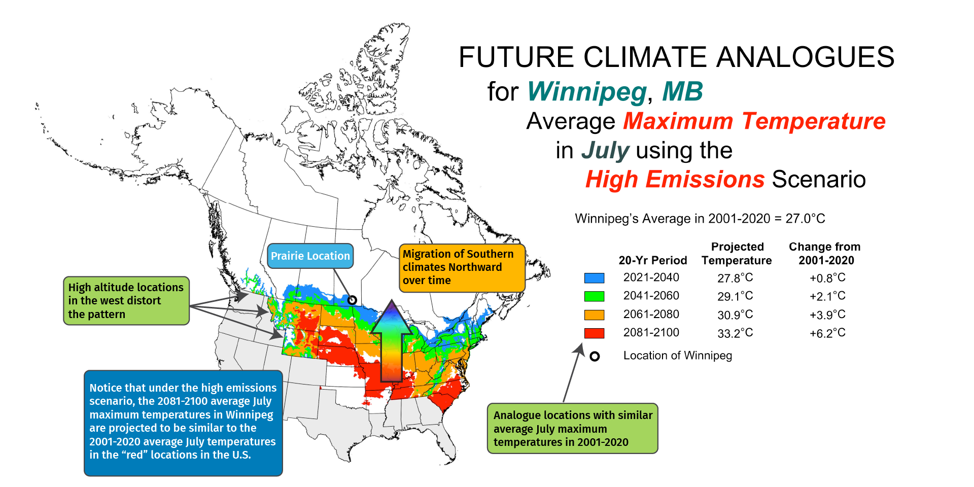
Also shown is a reminder that some of the analogues in the western states are related to the high altitude of the stations (relative to the altitude of the Prairie location).

The figure includes an example of how to interpret the pattern of the coloured analogue locations. It also has an arrow overlain on the figure to indicate that the placement of the coloured 20-year period areas further and further south over time indicates that the climates currently in the south are projected to 'migrate' northward over time, as the temperatures across the continent rise. The amount of migration varies by time of year, temperature variable, carbon scenario, and Prairie location.

One thing you will likely notice is that the migration distances are generally much larger in the warmer times of the year than in the colder times of the year. This is because the north-south temperature gradient in central North America is much larger in the winter than in the summer. That is, in the winter you don't have to go very far south across the 49th parallel to find average temperatures that are quite a bit higher than those in southern Canada, whereas in the summer you have to go much farther to find the same level of temperature change. To verify that this is the case, be sure to look at how a Prairie location's average temperature in the 20-year periods change over time. You will likely see that the temperature changes over time are quite large in the winter months, even though the migration distances might be quite small.

Limitation

The analogues presented here are, by design, simplistic. They only show analogues for temperature variables monthly, seasonally, and annually. And they do not attempt to identify analogues that consider how temperatures vary throughout the year, across the seasons – which are of course quite variable in southern Canada. Nor do they consider a very important aspect of all climates: precipitation.